Bitcoin as a Store of Value and Experiments with Algorithmic Trading Strategies

Introduction
Bitcoin (BTC) is proposed to provided a modern era store-of-value and be a potential successor to Gold (GLD)(Ammous, 2018).
Ammous (2018) illustrates that one of the key determinate factors of both BTC and GLD in conferring this property is that they both demonstrate a high stock-to-flow ratio.
Stock-to-flow refers to the property by which the current global stock or holding of an asset compares to the potential incoming flow of that asset. For example, the global stock of GLD compared to the potential new production of GLD is very high — i.e. its a rare metal on Earth and the effort of extraction of new GLD only accounts for some 2% of the stock. This is compared to the potential stock-to-flow of fiat currency whereby government issued paper (no longer backed by anything like a gold standard) can be printed / minted readily (with little effort) thus large quantities of new flow can devalue currently held stock, leading to inflationary periods and the consequential socio-economic results.
The economic model of BTC is purported to resemble that of GLD as BTC miners are effectively expending a larger amount of resource and effort in minting new Bitcoins. In addition the total global supply of BTC is capped to 22 million; this should result in a deflationary currency.
This study will make heavy use of the methods of Hilpisch (2020), who writes as a specialist in the domain of data-driven finance. So as such this post is both a learning exercise of personal interest in the crypto currency markets and a vehicle by which the author can learn and test the methods of Hilpisch.
Problem Statements
- Investigate the potential correlation between BTC and GLD returns in time-series, assuming a positive correlation indicates some representation whereby BTC is also considered a store-of-value. The assumption here is that when investors opt for gold as a store-of-value they could also opt for BTC.
- Machine learning will be applied to determine if the trades into BTC or GLD can be recommended over just holding a long position (it is suspected that the recent activities driving the price of BTC higher could result in an extremely simple, hold only strategy)
Metrics
The metrics for this project are relatively simple, given the strong connection to the financial domain and are either the price of the assets (GLD, BTC), the returns or relevant statistical metrics such as correlation.
Data
Data for crypto currency prices where obtained for free from https://www.cryptodatadownload.com and data is from the crypto currency exchange Binance.
Data for gold prices was obtained from Yahoo Finance https://uk.finance.yahoo.com.
Environment
The analysis was carried out using Jupyter and Python 3.x. The analysis notebook and list of required libraries in use are noted in the accompanying GitHub repository at https://github.com/rsiwicki/rock_dex/.
Part 1. Data Exploration and Investigating Store of Value
The project does not require a full Extract Transform Load (ETL) pipeline, however there is a need to extract and clean the data after a period of discovery. The extraction and initial analysis of daily BTC (from the exchange Binance (2021)) follows.
The raw data was in the form of a time-series of Open, High, Low, Close and additional information such as trade volumes and counts.
It appeared that there were null values for trade count. Upon inspection it seems that the missing values for trade count occur near the start of the data, assuming that Binance were not publishing these values during this time period. This was ameliorated later.
The data was visualised and analysed using Pandas upon import as a time-series. The first column (index_col=0), whilst representing the time-series is a Unix epoch time, we therefore re-imported the data using Pandas indicating that the date column (index_col=1) was the true indicator of the time-series. Pandas will automatically account for this and correctly build the time-series index (see Fig 1).

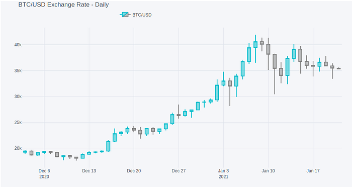
Visualisation of data often benefits from domain specific representations. In this case illustrating OHLC trade data using Candlestick charting (this originally was a Japanese method, used to help illustrate potential patterns in data that could result in new insight and trading strategies).
In this visualisation method the Open and Close prices are represented by the body of the candle (forming a box for each daily price quad). If the closing price is higher than the opening price the body of the candle is white, if the closing price is lower than the opening price the body colour is darker (in this case blue). The wicks of the candle represent the daily extremes of pricing. So the bottom line extending from the body is the lowest price experienced during the time period and the top line extending from the body is the highest price experienced for the period.
We will represent the OHLC data for BTC daily here using the Cufflinks Python library (recommended by Hilpisch, 2020) (see Fig 2).
In this next section we borrow some further techniques from Hilpisch (2020) to further illustrate relationships in the data to help convey information.
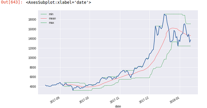
These techniques also explore our ability to use rolling window calculations in Python Pandas (see Fig 3).
- plotting mean max and average of closing prices.
- sub-plots of closing price, volumes and trade counts.
- applying a very simple fast-slow SMA strategy — to see if anything we produce using Machine Learning (ML) can out perform one of the most simple non-fundamental analysis strategies.
Subplots of the closing price, trade count and average trade size were also plotted. It was of interest to see if the average trade size was increasing with price.
It seems that the number of trades increased with price as did the average trade size. Though earlier trade sizes were also larger (driven by an unknown factor).
It seems that increased number of trades could represent liquidity and this liquidity could also increase the value of the asset.

In the section that follows we utilised a simple method from Hilpisch (2020) that utilises a fast and slow Simple Moving Average (SMA) to indicate Buy Sell signals. In this case when the Fast SMA trend-line moves over the Slow SMA trend-line a long position in BTC is proposed. The general trend of BTC has been to move upwards within this time frame, though as a basic signal this indicator looks like it would have been positive if somewhat simplistic.

We then followed to load the gold prices from Yahoo Finance (2021) and explore. Some further pre-processing of this data was required, particularly null values for certain days of the week.
It seems likely that the missing dates, predominantly Sundays, are holidays and the prices were not available to collect. Regardless of the reason to plot a chart, for example, would display breaks in continuity for these days. It seems reasonable to fill the missing data with that of the previous day to retain time series continuity. To achieve this we used the Pandas forward fill method of the fillna() function.
It was now possible to plot another simple SMA trading strategy chart for the GLD data to see how it differed from that of BTC.
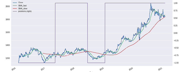
So already we can see a similarity between BTC and GLD. We then followed to plot the log of the return values for each asset (see Fig 7).
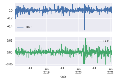
We can also follow the lead of Hilpisch (2020) and utilise ordinary least-squares (OLS) regression to determine the extent of correlation.
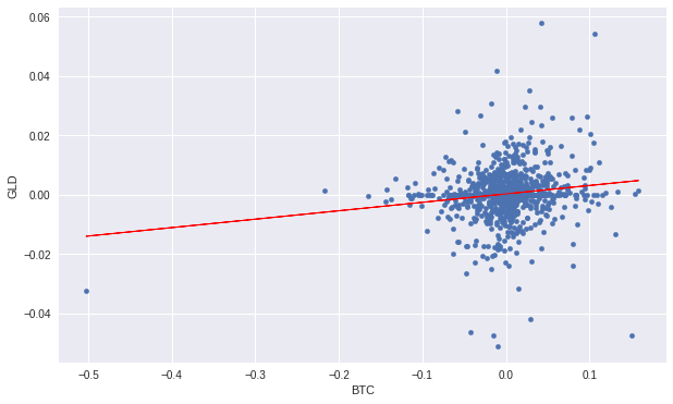
The correlation matrix can be demonstrated, thus:
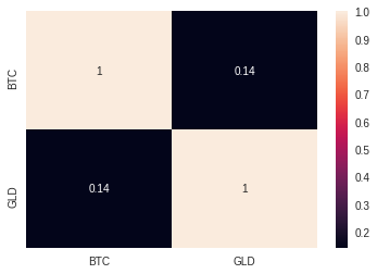
We can see that the correlation seems negligible.
Because the data is time series the correlation can be plotted over the time dimension to determine if there are periods where this correlation is stronger (See Fig 10).
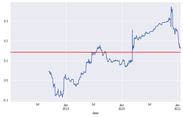
Correlation analysis over time series points to negative correlation prior to Jan 2020, thereafter positive. This however could be attributed to some other hidden factors or other global economic situations (speculation, though possibly the coronavirus pandemic). If the hypothesis at the outset were true, GLD and BTC should show some correlation if they are both considered stores of value. This does not appear to be the case prior to Jan 2020 though correlation seems to have increased after Jan 2020, though a continual trend upwards has been shown in the data set from the origin time. Regardless, the correlation is still weak at under 0.3, it would be interesting to follow the trend over time.
Does this increasing correlation really mean that BTC is becoming more like gold? Time could demonstrate that this correlation could potentially demonstrate the start of monetary competition with other stores-of-value.
Part 2. Trading Strategies and Machine Learning
In this section we return to the SMA example from earlier. We attempt to calculate the:
- Return of the simple SMA strategy over just holding a long position in the BTC asset.
- The possible enhancement of strategy that can be achieved using a simple machine learning model.
(We assume a trading period of 2018–01–03 to 2021–01–21 and cut the data this way to ensure a relevant cross over and complete inner join other than missing quoted days within the GLD price).
We calculated the log return of a hold only trading strategy for BTC and named this simple_returns. We then created a new measure, sma_returns to calculate the return determined by taking the short or long position indicated by utilising the SMA_slow and SMA_fast crossover (this is plotted as a dashed red line where -1.0 indicates short and 1.0 indicates long). The returns were also simulated by placing a trade at the close of day t0 and earning the returns of day t+1. The strategies are assuming no effect of trading costs, commissions or spreads (see Fig 11).
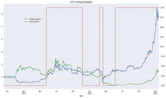
We can see that a simple SMA trading strategy would have been inferior to an even simpler holding strategy during the time period with the opportunity cost of 5.650317–1.389344 times the return.
In this section we prepared the model fit and evaluation technique as per Hilpisch (2020).
Data preparation to use the above strategies required that the returns in the data are classified as the log returns as per the previous calculations for the SMA trading strategy. The direction of the return also needs to be classified as to whether it is positive or negative. To do this we began to adjust the existing data from the SMA strategy above (see Fig 12).

Now the directions were classified according to the sign of the return.
We then engineered features for our algorithm’s input by using a lag of the returns following the methods of Hilpisch (2020). We choose six lags as the number of features; this is equivalent to a trader using six consecutive historical data points to predict the next movement direction of the currency. The output is illustrated below (see Fig 13).

The SVM is clearly outperforming other methods, quite substantially. Though this method is somewhat artificial as the entire data set it utilised. To test more realistic scenarios a test and train split of the data can be used. This will simulate training the data on historical returns and then using that to predict possible future returns on unseen data.
Splitting the data for this case is extremely simple and does not require the test_train_split function as it is merely time linear data. We chose a simple strategy outlined below to partition test and train data whereby train data was prior in the time-series to the split point and test data was future data by reference to the split point.
split_point = int(len(df_BTC_close_daily) * 0.3)
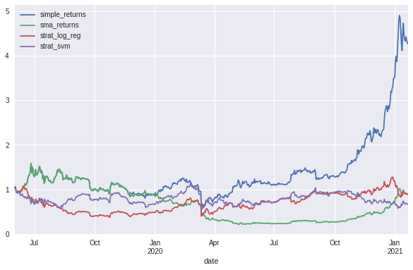
In this case where the algorithms are confronted with previously unseen data, no algorithmic machine learning strategy works better than a simple hold strategy.
Conclusion
Part 1 of this study, investigating how BTC could potentially relate to GLD as a store of value demonstrates that there is a possibility that there is an increasing correlation over time between BTC price and GLD price movements. To further improve this study, time is required to further assess the relationship in our existing simplified model; though, the addition and study of additional financial metrics that impact the GLD price, though applied to BTC could be considered — e.g. inflation metrics, bond yields etc.
Part 2 of this study deeply assessed the methods Hilpisch (2020) demonstrates in order to start identifying a potential machine learning based strategy for increasing hypothetical future returns of trading BTC, through only technical analysis and not fundamental analysis. The simple hold strategy was pitted against a second reference strategy of Fast and Slow Simple Moving Averages (SMA). Further to this Support Vector Machine and Logistic Regression strategies were added with simplified engineered features of return lags and whether a position should be short or long. The machine learning strategies all appeared to be weak once tested with a train / test split of the data and compared to a simple hold strategy.
Though our findings, that simply holding BTC generates effective returns and if in reality combined with costs accrued per trade, is certainly more efficient in the time period studied than employing a more sophisticated strategy; is perhaps itself a very fitting answer as to how best to trade BTC in the current environment: essentially buy and hold wins.
It is likely that the unusual nature of BTCs recent ascent could be confounding the training and testing of our algorithms: i.e. that the real driver for BTC prices is something more fundamental than technical analysis; such as the store-of-value effect studied in part 1.
Future improvement could include attempting the same strategies on hourly data instead of daily, perhaps here there are technical analysis relationships that are more subtle and intra-day trading could benefit from a machine learning approach. In addition hyper parameter tuning and adjusting the feature engineering to be more sophisticated combined with assessing different permutations of input features could be beneficial.
References
Ammous, S (2018). The Bitcoin Standard: The Decentralized Alternative to Central Banking. Wiley.
Binance (2021). Crypto Currency Data: Bitcoin USD. From https://www.cryptodatadownload.com.
Hilpisch, Y (2020). Python for Finance: Mastering Data Driven Finance. O’Reilly.
Yahoo (2021). Gold Prices Daily. From https://uk.finance.yahoo.com.
